39 how to add percentage data labels in excel bar chart
Excel Charts: How To Show Percentages in Stacked Charts (in ... - YouTube Download the workbook here: the full Excel Dashboard course here: h... How to show percentage in Bar chart in Powerpoint - Profit claims Steps to show Values and Percentage 1. Select values placed in range B3:C6 and Insert a 2D Clustered Column Chart (Go to Insert Tab >> Column >> 2D Clustered Column Chart). See the image below Insert 2D Clustered Column Chart2. In cell E3, type =C3*1.15 and paste the formula down till E6 Insert a formula3.
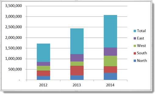
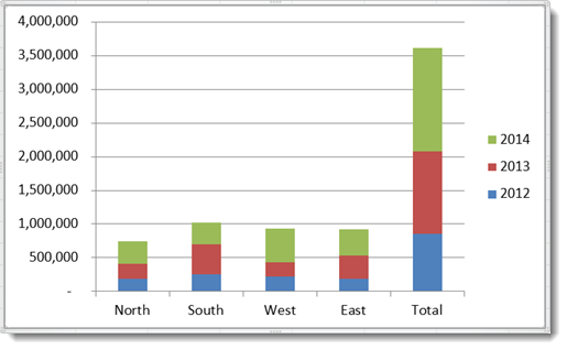
How to add total labels to stacked column chart in Excel? - ExtendOffice Select the source data, and click Insert > Insert Column or Bar Chart > Stacked Column. 2. Select the stacked column chart, and click Kutools > Charts > Chart Tools > Add Sum Labels to Chart. Then all total labels are added to every data point in the stacked column chart immediately. Create a stacked column chart with total labels in Excel
How to add percentage data labels in excel bar chart
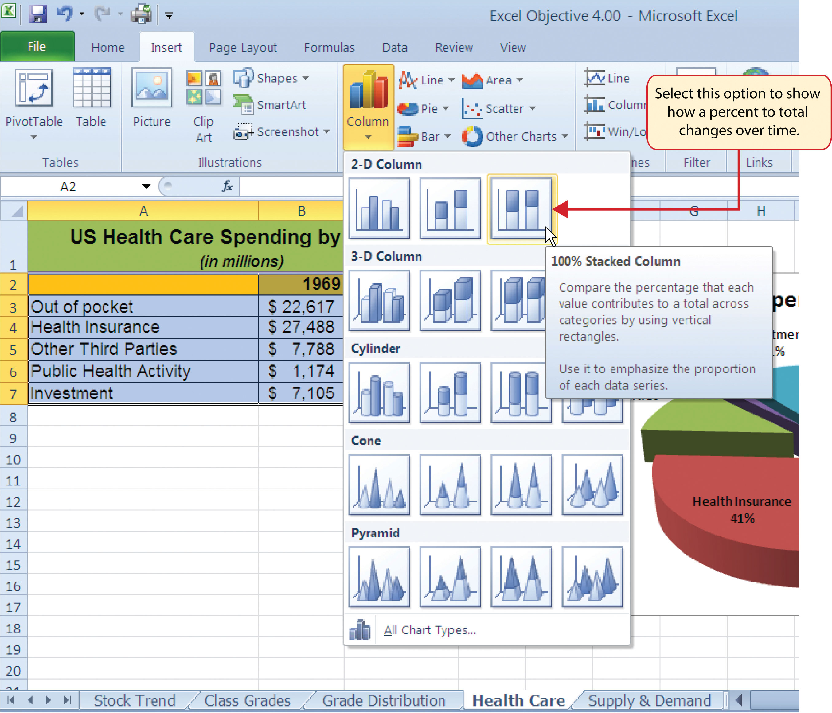
Data Bars in Excel (Examples) | How to Add Data Bars in Excel? - EDUCBA In order to show only bars, you can follow the below steps. Step 1: Select the number range from B2:B11. Step 2: Go to Conditional Formatting and click on Manage Rules. Step 3: As shown below, double click on the rule. Step 4: Now, in the below window, select Show Bars Only and then click OK. How to Show Percentages in Stacked Bar and Column Charts - Excel Tactics How to Show Percentages in Stacked Bar and Column Charts Quick Navigation 1 Building a Stacked Chart 2 Labeling the Stacked Column Chart 3 Fixing the Total Data Labels 4 Adding Percentages to the Stacked Column Chart 5 Adding Percentages Manually 6 Adding Percentages Automatically with an Add-In 7 Download the Stacked Chart Percentages Example File Create a column chart with percentage change in Excel - ExtendOffice Select the data in column C and column D, then click Insert > Insert Column or Bar Chart > Clustered Column to insert a column chart as below screenshot shown: 4. Then, press Ctrl + C to copy the data in column G, column H, column I, and then click to select the chart, see screenshot: 5.
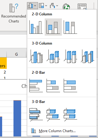
How to add percentage data labels in excel bar chart. How to Show Percentages in Stacked Column Chart in Excel? Follow the below steps to show percentages in stacked column chart In Excel: Step 1: Open excel and create a data table as below Step 2: Select the entire data table. Step 3: To create a column chart in excel for your data table. Go to "Insert" >> "Column or Bar Chart" >> Select Stacked Column Chart Step 4: Add Data labels to the chart. How to show data label in "percentage" instead of - Microsoft Community Select Format Data Labels Select Number in the left column Select Percentage in the popup options In the Format code field set the number of decimal places required and click Add. (Or if the table data in in percentage format then you can select Link to source.) Click OK Regards, OssieMac Report abuse 8 people found this reply helpful · How to Add Two Data Labels in Excel Chart (with Easy Steps) 4 Quick Steps to Add Two Data Labels in Excel Chart Step 1: Create a Chart to Represent Data Step 2: Add 1st Data Label in Excel Chart Step 3: Apply 2nd Data Label in Excel Chart Step 4: Format Data Labels to Show Two Data Labels Things to Remember Conclusion Related Articles Download Practice Workbook How to Add Percentages to Excel Bar Chart - Excel Tutorials To create a basic bar chart out of our range, we will select the range A1:E8 and go to Insert tab >> Charts >> Bar Chart: When we hover around this icon, we will be presented with a preview of our bar chart: We will select a 2-D Column and our chart will be created: Add Percentages to the Bar Chart
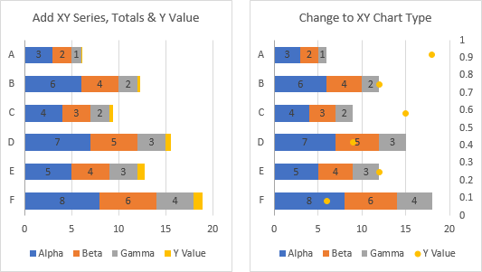
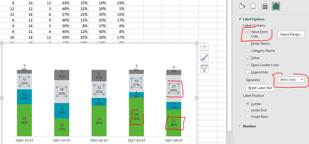
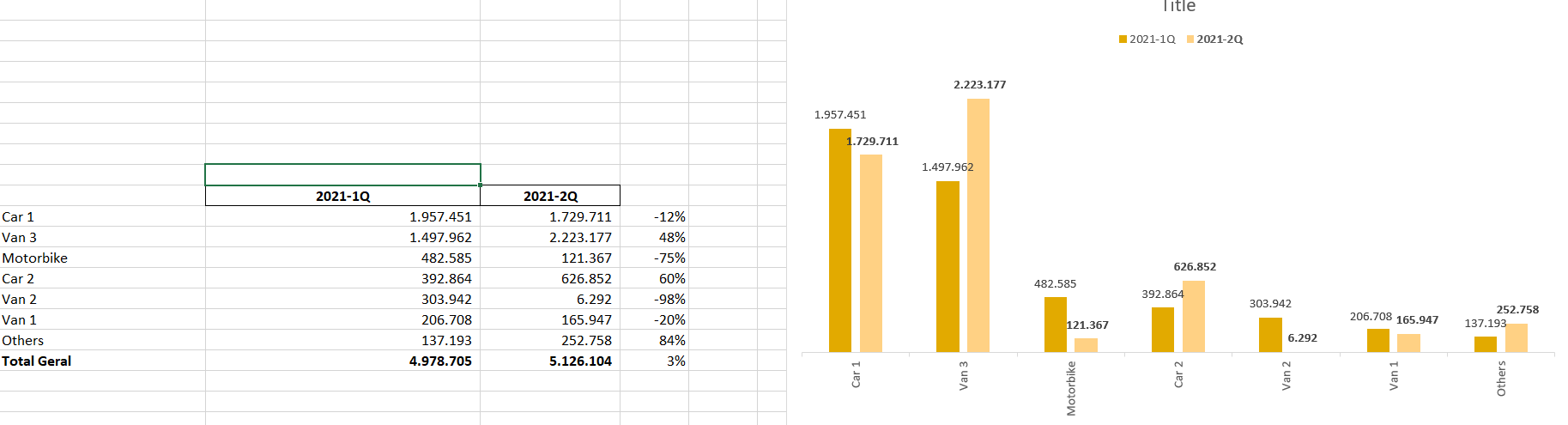
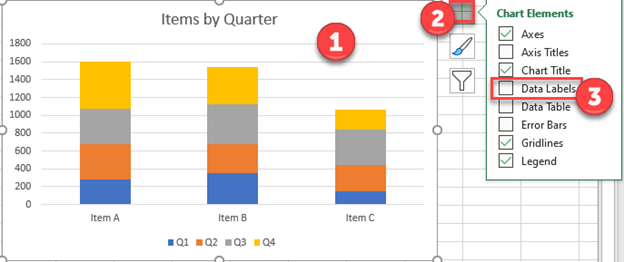
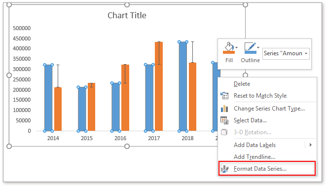
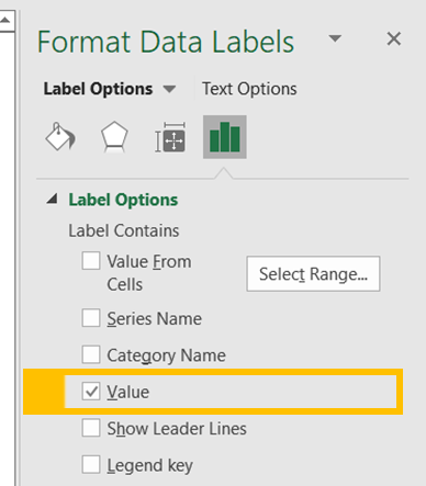
How to Make a Percentage Bar Graph in Excel (5 Methods) We will use it in our final method to produce a Percentage Bar Graph. Steps: Firstly, select the cell range C4:D10 and bring up the Insert chart dialog box as shown in method 2. Secondly, select the Funnel. Finally, press OK. This will output our Funnel Bar Graph. Moreover, we can format this Graph as shown in method 1 and method 2. Add or remove data labels in a chart - support.microsoft.com Click the data series or chart. To label one data point, after clicking the series, click that data point. In the upper right corner, next to the chart, click Add Chart Element > Data Labels. To change the location, click the arrow, and choose an option. If you want to show your data label inside a text bubble shape, click Data Callout. How to Show Percentage in Bar Chart in Excel (3 Handy Methods) - ExcelDemy Thirdly, go to Chart Element > Data Labels. Next, double-click on the label, following, type an Equal ( =) sign on the Formula Bar, and select the percentage value for that bar. In this case, we chose the C13 cell. In a similar fashion, repeat the process for the other values and finally, the results should look like the following. How can I show percentage change in a clustered bar chart? Double-click it to open the "Format Data Labels" window. Now select "Value From Cells" (see picture below; made on a Mac, but similar on PC). Then point the range to the list of percentages. If you want to have both the value and the percent change in the label, select both Value From Cells and Values. This will create a label like: -12% 1.729.711
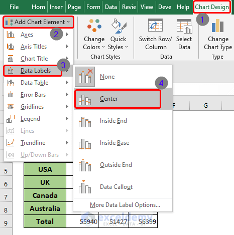
How to add percentage labels to top of bar charts? -Select all your data -Create the chart bar/line chart -Then select the line part of the chart and right-click -Choose show data labels - then delete the line -finally place the % labels where you want them to be... As i said this is an ugly way to do it, and there must be other's more elegant to do it, i'm shure, but this is what i can manage... How to show percentages in stacked column chart in Excel? - ExtendOffice Add percentages in stacked column chart 1. Select data range you need and click Insert > Column > Stacked Column. See screenshot: 2. Click at the column and then click Design > Switch Row/Column. 3. In Excel 2007, click Layout > Data Labels > Center . In Excel 2013 or the new version, click Design > Add Chart Element > Data Labels > Center. 4. How to show value and percentage in bar chart in excel With the data selected, click Insert > Column > Stacked Bar Chart; In the chart, right click on 'days since start' series bar by clicking onto the left half of the stacked bar. Then click Format Data Series in the drop-down menu, opening the side bar menu. Select No Fill under the Fill and Line tab. How to create a chart with both percentage and value in Excel? Click OK button, then, go on right click the bar in the char, and choose Add Data Labels > Add Data Labels, see screenshot: 12. And the values have been added into the chart as following screenshot shown: 13. Then, please go on right click the bar, and select Format Data Labels option, see screenshot: 14.
How to show percentages in stacked column chart in Excel?
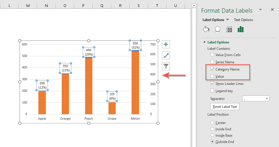
How to Display Percentage in an Excel Graph (3 Methods) Select Chart on the Format Data Labels dialog box. Uncheck the Value option. Check the Value From Cells option. Then you have to select cell ranges to extract percentage values. For this purpose, create a column called Percentage using the following formula: =E5/C5 The Final Graph with Percentage Change
Pie Chart Rounding in Excel - Peltier Tech
HOW TO CREATE A BAR CHART WITH LABELS ABOVE BAR IN EXCEL - simplexCT In the Format Data Labels pane, under Label Options selected, set the Label Position to Inside End. 16. Next, while the labels are still selected, click on Text Options, and then click on the Textbox icon. 17. Uncheck the Wrap text in shape option and set all the Margins to zero. The chart should look like this: 18.
Presenting Data with Charts
How to Add Percentage Axis to Chart in Excel - Excel Tutorials To do this, we will select the whole table again, and then go to Insert >> Charts >> 2-D Columns: To show percentages on a second axis, we first need to click anywhere on the orange bars that we have on our graph (this is not easy in this example as they are rather small). Once we do, we will right-click on it, and then select Format Data Series:
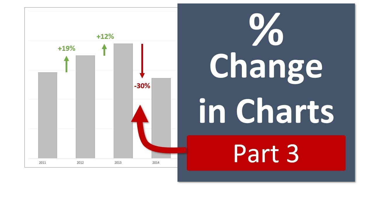
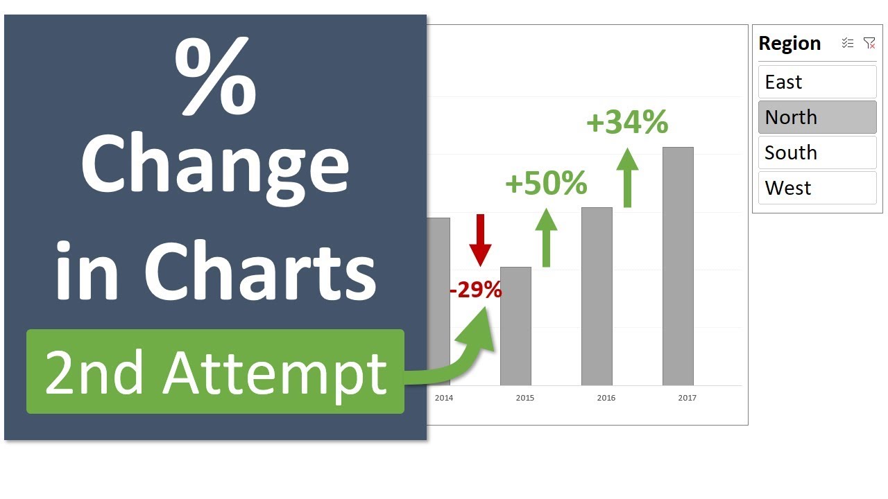
Column Chart That Displays Percentage Change - Part 3
Showing percentages above bars on Excel column graph Use a line series to show the % Update the data labels above the bars to link back directly to other cells Method 2 by step add data-lables right-click the data lable goto the edit bar and type in a refence to a cell (C4 in this example) this changes the data lable from the defulat value (2000) to a linked cell with the 15% Share
Add Totals to Stacked Bar Chart - Peltier Tech
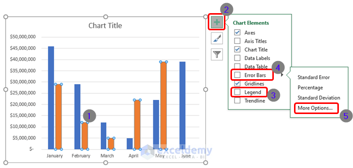
Change the format of data labels in a chart To get there, after adding your data labels, select the data label to format, and then click Chart Elements > Data Labels > More Options. To go to the appropriate area, click one of the four icons ( Fill & Line, Effects, Size & Properties ( Layout & Properties in Outlook or Word), or Label Options) shown here.
How to Show Percentages in Stacked Column Chart in Excel ...
HOW TO CREATE A BAR CHART WITH LABELS INSIDE BARS IN EXCEL - simplexCT 1. Highlight the range A5:B16 and then, on the Insert tab, in the Charts group, click Insert Column or Bar Chart > Clustered Bar. The chart should look like this: 2. Next, lets do some cleaning. Delete the vertical gridlines, the horizontal value axis and the vertical category axis. 3.
How to create a chart with both percentage and value in Excel?
How to show value and percentage in bar chart in excel On a chart , click the axis that displays the numbers that you want to format, or do the following to select the axis from a list of chart elements: Click anywhere in the chart . This displays the Chart Tools, adding the Design, Layout, and Format tabs.
Solved: Stacked bar graph with values and percentage (exce ...
How to Add Percentage or Count Labels Above Percentage Bar Plot scale_y_continuous(labels=percent) The plot from the first version is shown below. Add percentage labels to a stacked bar chart above bars. Lets try not to call our data "data", since this is a function in R! Using the data that I edited into your question. You can do what you would like by adding a geom_text that only looks at the data for ...

How to make a pie chart in Excel
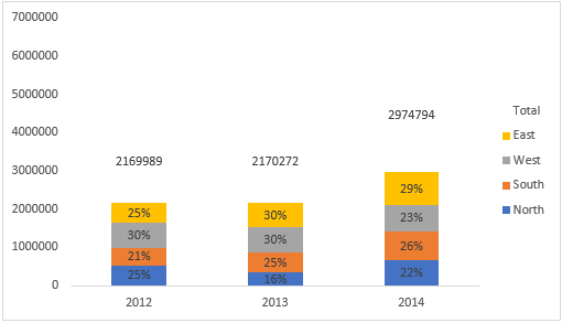
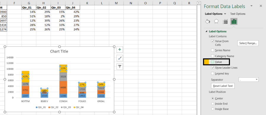
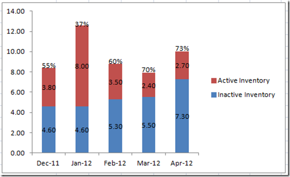
How to build a 100% stacked chart with percentages - Exceljet F4 three times will do the job. Now when I copy the formula throughout the table, we get the percentages we need. To add these to the chart, I need select the data labels for each series one at a time, then switch to "value from cells" under label options. Now we have a 100% stacked chart that shows the percentage breakdown in each column.
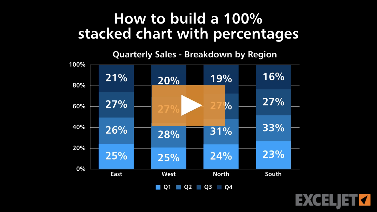
How to build a 100% stacked chart with percentages
How to add data labels from different column in an Excel chart? Please do as follows: 1. Right click the data series in the chart, and select Add Data Labels > Add Data Labels from the context menu to add data labels. 2. Right click the data series, and select Format Data Labels from the context menu. 3.
How can I show percentage change in a clustered bar chart ...
Create a column chart with percentage change in Excel - ExtendOffice Select the data in column C and column D, then click Insert > Insert Column or Bar Chart > Clustered Column to insert a column chart as below screenshot shown: 4. Then, press Ctrl + C to copy the data in column G, column H, column I, and then click to select the chart, see screenshot: 5.

How to make a pie chart in Excel
How to Show Percentages in Stacked Bar and Column Charts - Excel Tactics How to Show Percentages in Stacked Bar and Column Charts Quick Navigation 1 Building a Stacked Chart 2 Labeling the Stacked Column Chart 3 Fixing the Total Data Labels 4 Adding Percentages to the Stacked Column Chart 5 Adding Percentages Manually 6 Adding Percentages Automatically with an Add-In 7 Download the Stacked Chart Percentages Example File
Make a Percentage Graph in Excel or Google Sheets – Automate ...
Data Bars in Excel (Examples) | How to Add Data Bars in Excel? - EDUCBA In order to show only bars, you can follow the below steps. Step 1: Select the number range from B2:B11. Step 2: Go to Conditional Formatting and click on Manage Rules. Step 3: As shown below, double click on the rule. Step 4: Now, in the below window, select Show Bars Only and then click OK.
How to Add Percentages to Excel Bar Chart – Excel Tutorials

Solved: Clustered column chart - show percentage and value ...
How-to Put Percentage Labels on Top of a Stacked Column Chart ...
How to Show Percentages in Stacked Bar and Column Charts in Excel

Add Total Values for Stacked Column and Stacked Bar Charts in ...
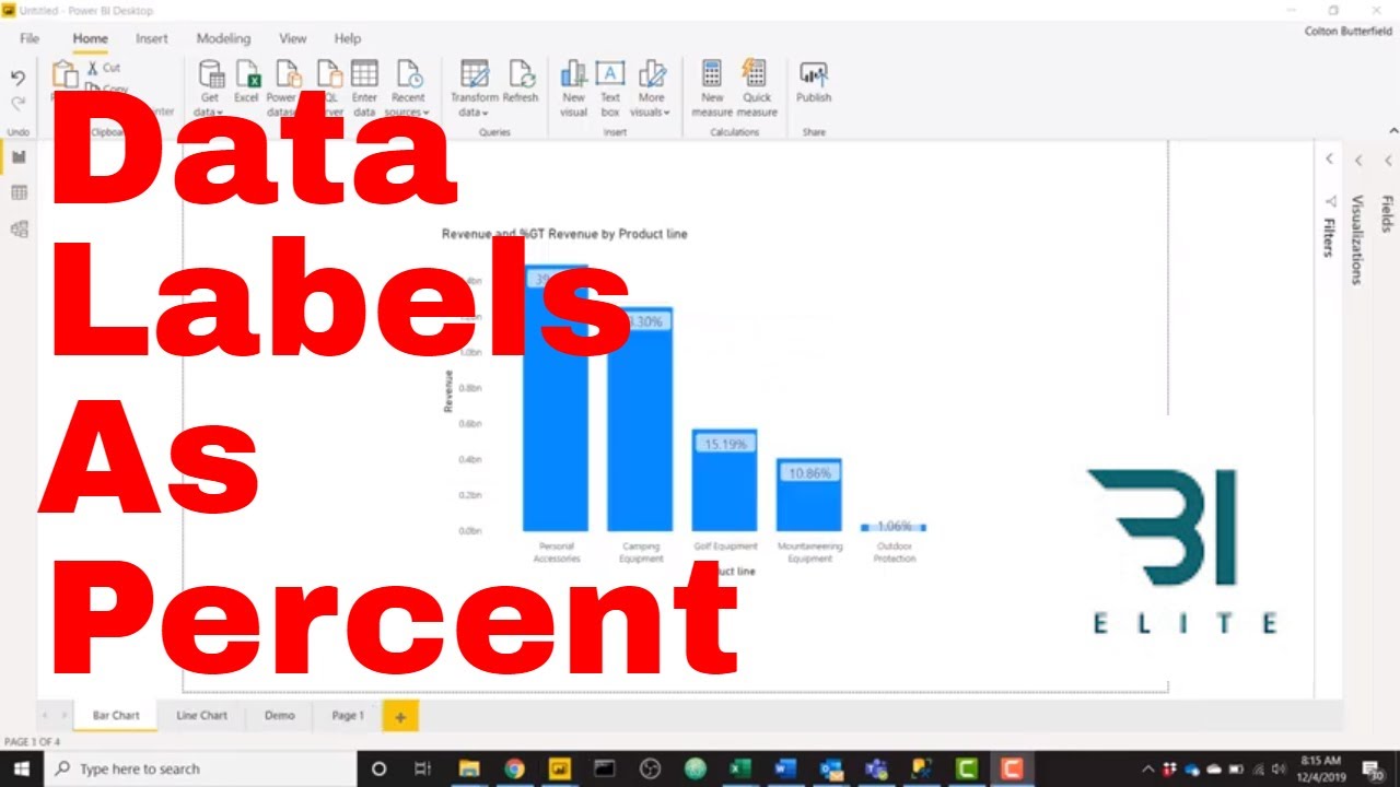
Power BI - Showing Data Labels as a Percent

Format Number Options for Chart Data Labels in PowerPoint ...
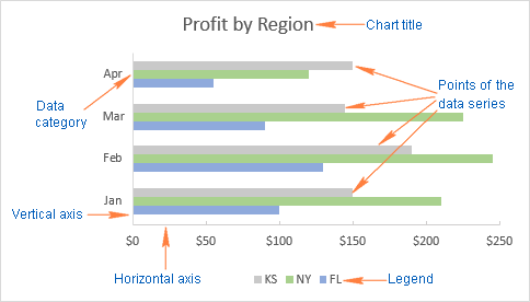
How to make a bar graph in Excel

How to create a chart with both percentage and value in Excel?

Add data labels and callouts to charts in Excel 365 ...
How to Display Percentage in an Excel Graph (3 Methods ...
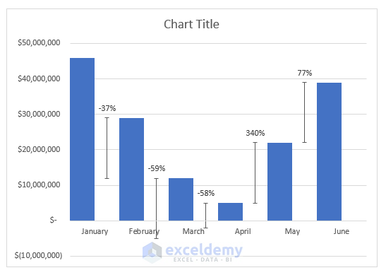
Percentage Change in Excel Charts with Color Bars - Part 2

Add Total Values for Stacked Column and Stacked Bar Charts in ...

Best Excel Tutorial - Chart with number and percentage
How to Add Percentages to Excel Bar Chart – Excel Tutorials

Add Percentage Labels to a 100% Stacked Bar chart in MS ...
Step by step to create a column chart with percentage change ...
How to Display Percentage in an Excel Graph (3 Methods ...

Change the format of data labels in a chart
Percent charts in Excel: creation instruction
Presenting Data with Charts
How to Show Percentages in Stacked Column Chart in Excel ...

Is there a way to add data labels as percentages on the ...
How to Display Percentage in an Excel Graph (3 Methods ...
How to Show Percentages in Stacked Bar and Column Charts in Excel

How to Add Data Labels to your Excel Chart in Excel 2013
Post a Comment for "39 how to add percentage data labels in excel bar chart"