44 excel pivot table conditional formatting row labels
Conditional Formatting on Pivot Table row labels As per my knowledge, in this case it does not matter what is the source of pivot as after getting the data in pivot, it's the pivot where the conditional formatting need to be applied, please upload a sample. thanks. Regards, DILIPandey DILIPandey +91 9810929744 dilipandey@gmail.com Register To Reply Overwrite pivot table conditional format based on row label As far as I know, using the one rule in the Conditional formatting, we can only format the cells with one color if the condition is true and if the same condition is false, the formatting of the cell will be blank and if both conditions are true, the formatting of cell depends on the highest ranking/priority of the rules in Conditional formatting.
Conditional Format Pivot Table Row | Chandoo.org Excel Forums - Become ... Select the entire row, and when you apply the conditional format, make the column reference absolute. So, say we want the entire row 2 to be formatted if cell in col B = 5. formula would be: =$B2=5

Excel pivot table conditional formatting row labels
Design the layout and format of a PivotTable To change the layout of a PivotTable, you can change the PivotTable form and the way that fields, columns, rows, subtotals, empty cells and lines are displayed. To change the format of the PivotTable, you can apply a predefined style, banded rows, and conditional formatting. Windows Web Mac Changing the layout form of a PivotTable Pivot Table Conditional Formatting - Contextures Excel Tips We'll adjust the formatting range, to fix that problem. Select any cell in the pivot table. On the Ribbon's Home tab, click Conditional Formatting, then click Manage Rules. In the list of rules, select the Data Bar rule, which applies to cells B3:B8. Click Edit Rule, to open the Edit Formatting Rule window. How to make row labels on same line in pivot table? - ExtendOffice Make row labels on same line with PivotTable Options You can also go to the PivotTable Options dialog box to set an option to finish this operation. 1. Click any one cell in the pivot table, and right click to choose PivotTable Options, see screenshot: 2.
Excel pivot table conditional formatting row labels. Pivot Table: Pivot table conditional formatting | Exceljet Select any cell in the data you wish to format and then choose "New rule" from the conditional formatting menu on the Home tab of the ribbon. At the top of the window, you will see setting for which cells to apply conditional formatting to. For the example shown, we want: "All cells showing sum of "sales values" for name and "date" Conditional formatting rows in a pivot table based on one rows criteria ... What you need to do is accept the formula the way you type it, close the conditional formatting rules manager and then reopen it. Remove the $ from the row numbers that excel added into your formula but leave it on the column number like so =$I3=992, or whatever your first row is. conditional formatting per row on pivot - Microsoft Tech Community conditional formatting per row on pivot. I would like to format each row of a pivot table separately (as in the picture shown below), but I cannot paste the formatting. I've got many rows, and they could change (just like the columns) Is there a way to automate this, or I have to select row by row and apply the formatting? Pivot Table Conditional Formatting - Microsoft Tech Community Hi all :) I have an issue conditionally formatting a Pivot Table. I have my row hierarchy set up as Region, Area, Store, Consultant. My rows are expanded out only to a Store Level. I need the Store Name to be highlighted red if the value in the first column is <1. I have applied conditional fo...
Conditional formatting for Pivot Tables in Excel 2016 - 2007 - Ablebits The format I used was to select Conditional Formatting > Top 10 Items > set it to 1 item and select the default format. This format can be copied from one range to the next if desired or built up for each range individually. To copy the format, select one or more cells with that format and click Copy. Apply Conditional Formatting | Excel Pivot Table Tutorial Go to Home Tab → Styles → Conditional Formatting → New Rule. From rule to, select the third option. And, from "select a rule" type select "Format only top or bottom" ranked values. In edit rule description, enter 1 in the input box and from the drop-down menu select "each Column Group". Apply formatting you want. Click OK. Format Pivot Table Labels Based on Date Range Select all the dates in the Row Labels that you want to format. On the Ribbon, click the Home tab, and then in the Styles group, click Conditional Formatting. In the list of conditional formatting options, click Highlight Cells Rules, and then click A Date Occurring. Highlight Cell Rules based on text labels | MyExcelOnline Pivot Tables in Excel are one of the most powerful features within Microsoft Excel that allows you to analyze more than 1 million rows of data with just a few mouse clicks. You can use conditional formatting with Excel Pivot Tables to highlight cell rules based on text labels. Let me show you how easy this is with the help of examples.
Pivot Table Conditional Formatting - Computer Tutoring Because we selected this cell the Conditional Formatting will apply to the month grouping level. The month grouping level is indicated by the work date in the Rows section of the Pivot Table.) From the Home Tab in the Styles section choose Conditional Formatting - Highlights Cells Rules - Less Than. In the Less Than box type 90% then click OK. Excel Conditional Formatting in Pivot Table - EDUCBA Click on any cell in the pivot table > Go to the HOME tab > Click on Conditional Formatting option under Styles option > Click on Manage Rules option. It will open a Rules Manager dialog box. Click on the Edit Rule tab, as shown in the below screenshot. It will open the Editing Rule formatting window. Refer to the below screenshot. Excel VBA: Conditional Format of Pivot Table based on Column Label ... myPivotSourceName = myPivotField.Name. Then rather than referencing the data field with the pivot field object, I referenced the DataRange with the string: myPivotTable.PivotFields (myPivotSourceName).DataRange.Select. Works perfectly and is completely portable for any pivottable on any sheet with any fields. excel vba. Pivot Table Conditional Formatting Based on Another Column ... - ExcelDemy We can conditionally format the entire Pivot Table depending on the blanks. Step 1: Repeat Step 1 of Method 1 then the New Formatting Rule window will open. Here in the New Formatting Rule window, Select the 3rd and 2nd options from Apply Rule to and Select a Rule Type command box respectively. Inside Edit the Rule Description dialog box,
85 DOWNLOAD PRINTABLE HOW DO I PIVOT TABLE IN EXCEL PDF DOC ZIP - Pivot
Pivot Table Conditional Formatting with VBA - Peltier Tech sub formatpt1 () dim c as range with activesheet.pivottables ("pivottable1") ' reset default formatting with .tablerange1 .font.bold = false .interior.colorindex = 0 end with ' apply formatting to each row if condition is met for each c in .databodyrange.cells if c.value >= 7 then with .tablerange1.rows (c.row - .tablerange1.row + 1) …
Sorting a Pivot Table | MyExcelOnline
How to Apply Conditional Formatting to Pivot Tables - Excel Campus Bottom Line: Learn how to apply conditional formatting to pivot tables so that the formats are dynamically reapplied as the pivot table is changed, filtered, or updated. Skill Level: Intermediate Download the Excel File. Here's the file that I use in the video. You can use it to practice adding, deleting, and changing conditional formatting on a variety of pivot table examples.

How To Find And Remove Duplicates In A Pivot Table - MS Excel | Excel In Excel
How to Highlight A row based on Cell Value In Pivot Table Basically, pivot tables were used to summarize a huge data. Meanwhile, conditional formatting is used to highlight a value with a logical connection. But, Can a particular cell value gets highlighted using conditional formatting?. This article provides the user with inputs required to highlight a row based on cell value in pivot table.
Finding Duplicates by Using Conditional Formatting in Excel 2010
Pivot Table Conditional Formatting for Different Rows Items? Select Your Pivot Table and: Go to Conditional Formatting -> New Rule -> Choose All cells showing "duration" values for "Type and "Date Selection" under "Apply Rule To" section -> Use a Formula to Determine which cells to format and enter the following formula: =AND(A6="Cars",A6>3), You can create new rules for other two conditions as well:

Pin by Larry Xu on Excel | Pivot table, Excel, Row labels
How to Apply Conditional Formatting to Rows Based on Cell Value - Excel ... On the Home tab of the Ribbon, select the Conditional Formatting drop-down and click on Manage Rules…. That will bring up the Conditional Formatting Rules Manager window. Click on New Rule. This will open the New Formatting Rule window. Under Select a Rule Type, choose Use a formula to determine which cells to format.

Pivot Tables – Excel Tips and Tricks
How to apply conditional formatting to Pivot Tables - SpreadsheetWeb Go to HOME > Conditional Formatting > New Rule to add a new formatting rule, or select from predefined options. If you select the latter, you will need to configure the rule regardless. The New (or Edit) Formatting Rule window contains options specific to Pivot Tables. You can choose the location where you want to apply your conditional ...

How To Find And Remove Duplicates In A Pivot Table - MS Excel | Excel In Excel
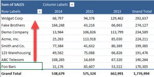
Conditional Formatting in Pivot Table - WallStreetMojo Currently, a pivot table is blank. Next, we need to bring in the values. Then, drag down the "Date" in the "Rows" Label, "Name" in the "Column," and "Sales" in "Values." As a result, the pivot table will look like the one below. To apply conditional formatting in the pivot table, first, we must select the column to format.

33 Pivot Table Blank Row Label - Labels Database 2020
Apply conditional formatting for each row in Excel - ExtendOffice 3. Click Format button to go to the Format Cells dialog, and then you can choose one formatting type as you need. For instance, fill background color. Click OK > OK to close dialogs. Now the row A2:B2 is applied conditional formatting. 4. Keep A2:B2 selected, click Home > Conditional Formatting > Manage Rules.
Post a Comment for "44 excel pivot table conditional formatting row labels"